Training Neural nets through BatchNorm: Challenging a 2015 study
Understanding the what and why of Batch Normalization

By Mahendra Kariya
In 2015, a couple of researchers from Google came up with the idea of batch normalization. It quickly gained popularity and is used very widely today, in the real world as well as in research (7000+ citations in less than 3 yrs). After all, BatchNorm makes it easier to train neural nets. The primary reasons for this were:
- With batch normalization, we can use higher learning rates.
- It reduces the dependence of gradients on their initial values, which means, weight initialization becomes easier.
- It even acts as a regularizer and reduces the need to use other regularization techniques.
- It also enables usage of saturating non-linearities.
All in all, this results in faster training.
In the original paper, the authors claim that batch normalization improves training performance by reducing internal covariate shift. This has also been the popular explanation in deep learning literature. However, in Oct 2018, a bunch of researchers from MIT ran some experiments and claimed that this is not the case. (They are presenting this research in NeurIPS 2018.) In this particular post, we will give a brief overview of what this technique is, the original intuition behind it and the subsequent experiments run by MIT researchers. Broadly, we will discuss the main points of the following two research papers.
- Batch Normalization: Accelerating Deep Network Training by Reducing Internal Covariate Shift, by Sergey Ioffe and Christian Szegedy. arXiv: 1502.03167, 2015
- How Does Batch Normalization Help Optimization?, by Shibani Santurkar, Dimitris Tsipras, Andrew Ilyas, and Aleksander Madry. arXiv: 1805:11604, 2018
Data Distribution Similarity
As Data Scientists, we all understand the importance of ensuring the distribution of the input data stays more or less similar during training and inference time. If the distribution changes at inference time, our model is bound to fail. This particular phenomenon where the distribution of data changes is called covariate shift. One of the ways we avoid covariate shifts is by retraining the model frequently on newer data.
Covariate Shift and Neural Networks
A neural network is made up of a bunch of layers. And inputs to each layer is nothing but the output of the previous layer, except for the input layer. During the course of training, the distribution of the input data to a particular layer changes as the previous layers learns new weights due to the back propagated error. As a result, various layers try to learn the representations from data whose distribution is continuously changing. This is what Sergey Ioffe and Christian Szegedy call internal covariate shift.
Training Deep Neural Networks is complicated by the fact that the distribution of each layer’s inputs changes during training, as the parameters of the previous layers change. We refer to this phenomenon as internal covariate shift.
— Ioffe and Szegedy (https://arxiv.org/pdf/1502.03167.pdf)
Normalization to the rescue
Normalization is a pretty common technique in Machine Learning. We generally normalize the input data before feeding it into any model. This helps gradient descent achieve faster convergence. Some normalization techniques also change the distribution of input data so it has zero mean and unit variance.
Batch Normalization
With this intuition in mind, Ioffe and Szegedy came up with the idea of Batch Normalization. They claim if the layer inputs are normalized to have zero mean and unit variance, the problem of interval covariate shift can be solved.
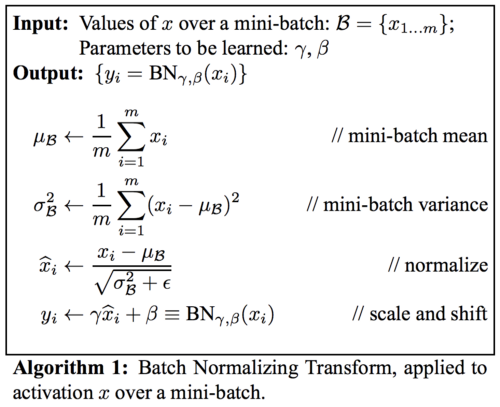
The figure on the left is the batch normalization algorithm given in the paper. It’s pretty straight forward. We take the mean and variance of the activations of the previous layer (inputs to the current layer) for each mini batch and use it to normalize them. This is very similar to how we normalize the input data.
But let’s focus on the last line. We may not always want zero mean and unit variance. Hence, the authors have introduced two learnable parameters, γ and β. We generally initialize these parameters to transform the data to zero mean, unit variance distributions. But during the course of training, they can learn any other value that might be better.
Implementing BatchNorm
Implementing batch normalization is super easy. Most of the famous deep learning frameworks have an API (TF, Keras, PyTorch, MXNet) that lets us implement it with just a single line of code. However, for those who would like to implement it from scratch, there is a nice blog post written by Frederik Kratzert you can refer.
If you’d like to go in a bit more detail about the intuition and the reason given by the original authors, take a look at the following video by Andrew Ng.
Is Internal Covariate Shift Important?
Until now, this was our understanding of batch normalization. But Shibani Santurkar, Dimitris Tsipras, Andrew Ilyas, and Aleksander Madry questioned the basic intuition behind internal covariate shift. Is controlling the mean and variance of distributions of layer inputs directly connected to improved training performance?
To answer this question, they ran an experiment. They created three variants of VGGNet and trained it on CIFAR-10. The first variant is standard VGGNet. In the second variant, they added BatchNorm layers. In the third variant, they injected random noise after the BatchNorm layer. Each activation of each sample was perturbed with i.i.d. noise sampled from a non-zero mean and non-unit variance distribution. This noise distribution changed at every step. Such noise injection introduced a severe covariate shift. The following figure visualizes the performance of the three variants of VGGNet.
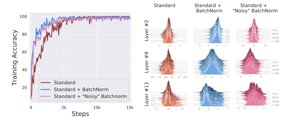
Looking at the above figure, it’s quite clear that the performance difference between the BatchNorm and the noisy BatchNorm variant isn’t significant. The variant without BatchNorm doesn’t perform as well as the other two. The figure on the right hand side shows the distributions of the three variants at different layers in the network.
It is clear from this experiment that even with internal covariate shift, a network can have improved training performance. In this experiment, the authors also added the same amount of noise to the first variant of VGGNet (without BatchNorm). This prevented the network from training entirely. This reinforces our current understanding that BatchNorm is indeed important.
So far, we have two conclusions:
- BatchNorm is important. It certainly helps in improving the training performance.
- However, the performance improvement provided by BatchNorm isn’t due to the stabilisation of mean and variance of layer inputs.
Expanding the scope of internal covariate shift
So far, we have only considered the mean and variance of the distribution to describe internal covariate shift. Let’s expand this definition.
In a neural network, each layer can be considered as solving an empirical risk minimisation problem. Each layer optimizes some loss functions (along with other layers). Changing the inputs to these layers implies that we are changing the empirical risk minimisation problem itself. And this happens all the time in a neural net. Given that BatchNorm primarily improves the optimization speed, we can add a broader notion to the definition of internal covariate shift; something that is more closely related to the optimization task.
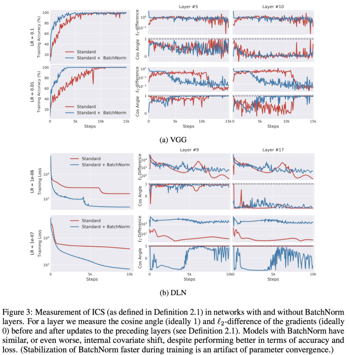
The parameter updates happen based on the gradient of the loss function. We can quantify the amount of adjustment the parameters go through in reaction to parameter updates in previous layers by taking the difference between the gradients of all the layers before and after the updates to its previous layers. So, let gᵢ represent the gradient of parameters that will be applied normally, and 𝔤ᵢ represent the same gradient after all previous layers have been updated. We can define internal covariate shift as the norm of the difference between gᵢ and 𝔤ᵢ. Internal covariate shift = ‖gᵢ - 𝔤ᵢ‖₂.
Based on our understanding so far, we should expect that addition of BatchNorm will reduce internal covariate shift, by increasing the correlation between gᵢ and 𝔤ᵢ.
Santurkar et al. ran this experiment and found the exact opposite. Networks with BatchNorm layers often exhibit no correlation between gᵢ and 𝔤ᵢ, and result in an increase in internal covariate shift. This is in spite of the case that networks with BatchNorm perform significantly better in terms of accuracy and loss. Refer the below figure below to see the results of this experiment.
What makes BatchNorm work?
So far, we have seen that BatchNorm really works well. But our reasoning behind its improved performance is wrong. So what is it that makes BatchNorm work so well? Before we get into the details of this, let’s take a slight detour and visit the optimization-land.
Detour to the optimization-land
Neural networks generally use some variant of SGD. And we are well aware of the fact that the shape of the loss function plays a significant role in how the optimization goes. The rockier the loss function, the harder it is to optimize. Similarly, the path to convergence is easier in a smoother loss function.
The smoothness of any function can be defined by its Lipschitz constant, named after German mathematician Rudolf Lipschitz. Lipschitz continuity is a strong form of uniform continuity for functions. The concept of Lipschitz continuity is very well explained on Wikipedia. It goes as follows:
Intuitively, a Lipschitz continuous function is limited in how fast it can change: there exists a real number such that, for every pair of points on the graph of this function, the absolute value of the slope of the line connecting them is not greater than this real number; the smallest such bound is called the Lipschitz constant of the function.
In simple terms, we can think of the Lipschitz constant as a measure of how fast a function can change. A function with a Lipschitz constant L is called L-Lipschitz. And a function is considered β-smooth if its gradients are β-Lipschitz. If you’d like to read more about Lipschitzness, take a look at this math stackexchange question.
Back to the original question
Let’s get back to our original question. What makes BatchNorm work? To answer this question, Santurkar et al. analyzed the optimization landscape of the network with and without BatchNorm. They found that BatchNorm makes the optimization landscape much more smoother. This means that BatchNorm improves the Lipschitzness of the loss function. They even found out that BatchNorm improves the Lipschitzness of the gradients of the loss function as well. This means that the loss exhibits significantly better effective β-smoothness. See figure below.
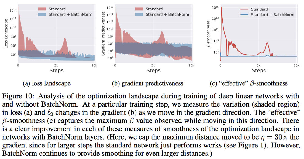
Because our optimization landscape is now much more smoother, we can take a larger step in the direction of the gradient, without the fear of getting trapped in a local minima or a plateau region. Hence, we can use larger values of learning rates. As a result, the training becomes faster and less sensitive to hyper parameter choices. This explains the benefits of BatchNorm, that we discussed in the beginning of this post.
The following short 3 minute video summarizes this idea. Alternatively, take a look at this poster.
At GO-JEK, we continuously believe in improving our craft. The good thing about working with GO-JEK; we can all dedicate 20% of our time to play around with projects outside our typical scope of work. This helps us immensely and keeps us up to date with interesting, cool things researchers put out. That’s my pitch if you ever wanted to join GO-JEK. Grab the chance, you might be missing out on working with some of the most passionate people out there. Check out gojek.jobs for more.