Fantastic drivers and how to find them

By Ishita Mathur

Problem Statement

A POI, or Place of Interest, in our context, is defined as a place where a high number of pickups happen. This can be at any popular location, such as a mall, train station, or even a large residential complex. In the earlier versions of our app, when a user booked a GO-RIDE or a GO-CAR at a POI, they had to coordinate with the driver to confirm the exact pick up point: the experience we were offering drivers and customers was less than adequate.

We wanted to decrease this friction by letting the user choose the exact ‘gate’ or entrance they would want to be picked up from. The allocated driver would then directly arrive at that point without the need to coordinate over calls or chat messages. But how would we know where these gates, i.e. convenient or popular pickup spots should be?

One way of doing this was to manually identify popular pick up spots. But this was undoubtedly an unscalable approach, given the number of POIs we want to solve this problem for.

It’s also not in GO-JEK’s engineering team to manually do things that can easily be automated. 😉

Our Solution

In order to scale, we had to automate this process, i.e., build an algorithm that can correctly identify the clusters of popular pickup points the same way a human brain intuitively does, by looking at the plots manually.

To do this, we took advantage of historical data we had about where exactly customers were being picked up from around such POIs. Below is a sample of pickups locations from where customers have been picked up around Blok M Square, a mall in Jakarta.

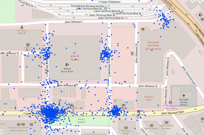
From the image, it’s fairly obvious to the human eye that there are five regions around the mall where pickups most frequently happen. But how would we determine this in an automated fashion?

We had to build an algorithm that can not only correctly identify separate clusters from each other, but also allocate a central point for each cluster that best represented where pickups frequently happen.

Clustering Algorithms

We experimented with various clustering algorithms, of which we’ll discuss DBSCAN and KMeans. While both are unsupervised algorithms, the former is a density-based clustering algorithm that effectively removes noise, and the latter is a distance-based that does not account for noise in the dataset.

This section will talk about why we chose the latter, and how we worked around its shortcomings.

DBSCAN

For DBSCAN to work effectively, clusters need to have similar densities and cannot be scattered; any data point will be considered an outlier if it is further than the distance metric, eps, from the other data points.

The geospatial pickup data we were dealing with contained both of the following extremes:

• If a particular pickup spot around a POI can be more widely preferred and consequently have a higher density. This means that a pickup cluster can have a density that is higher or lower than other clusters for that POI.
• Scattered pickup locations can always occur if GPS accuracy of the device is low. This would mean that any pickup cluster in a building’s basement, or one with slightly scattered pickups, would not even be considered as a cluster.

As was evident from the data, the actual conditions were far from ideal when it came to the requirements for DBSCAN. The density of pickups will almost always be different across different POIs, and is likely to be different across pickup clusters within the same POI as well. Keeping this in mind, generalising the DBSCAN algorithm across POIs would be difficult.

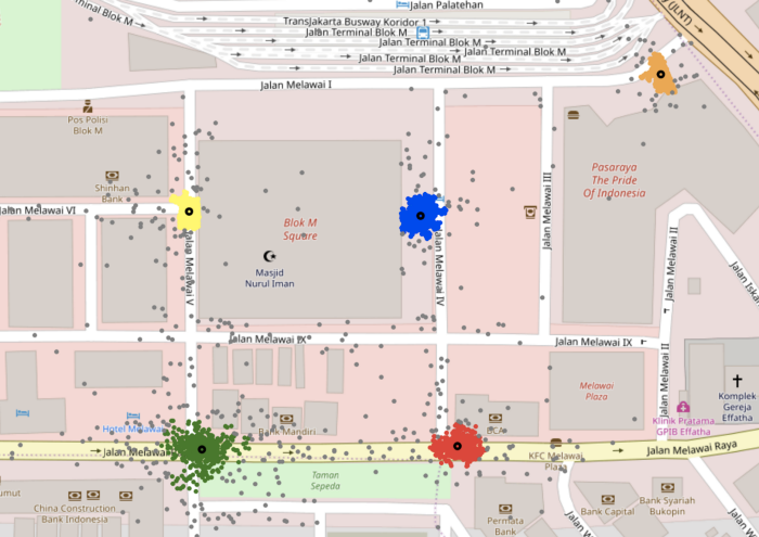
In the example of Blok M Square below, the algorithm (after some hyperparameter tuning) was able to identify the clusters and the outliers (points indicated in grey) as the density of pickups in all 5 gates is somewhat uniform.

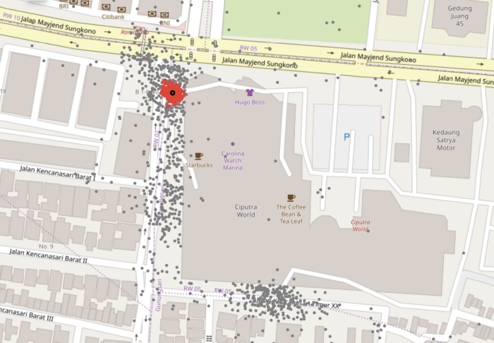
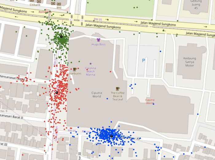
However, as the pickup points for some gates are more spread out, DBSCAN was unable to generalise well to another mall, Ciputra World, as can be seen in the image below.

KMeans

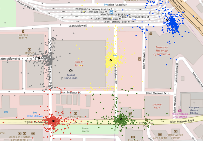
KMeans is a distance-based clustering algorithm, where each point is assigned to the nearest cluster centre. Although the algorithm doesn’t account for outliers, it was much more effective in correctly identifying the clusters that DBSCAN was unable to, as is evident from the images below. For Ciputra World, it correctly identified the three clusters while DBSCAN was unable to identify two of the clusters as the pickups in the area were relatively scattered.

However, KMeans has one major drawback: k, or the number of clusters, needs to be an input to the model. Next, we needed to automate the process of accurately determining the value of k for each POI.

Approach 1: Diving bookings by s2 cells

The initial approach that was taken involved dividing all the bookings for a single POI into Level 17 S2 cells (each of which has a width of approximately 70 metres) and assume two clusters (i.e., take k=2) in each cell. Since an S2 cell boundary might exist in the middle of a cluster, this would equate to the algorithm considering the cluster as two separate ones; one in each of the neighbouring cells. Thus a subsequent de-duplication step would be required to combine any two clusters having cluster centres that were closer than 25 metres from each other.

There were several problems with this approach — the primary one being that the threshold distance for deduplicating clusters was arbitrary and could not be generalised across all POIs. This is because cluster sizes greatly varied between POIs.

Approach 2: Analytical computation of ‘k’

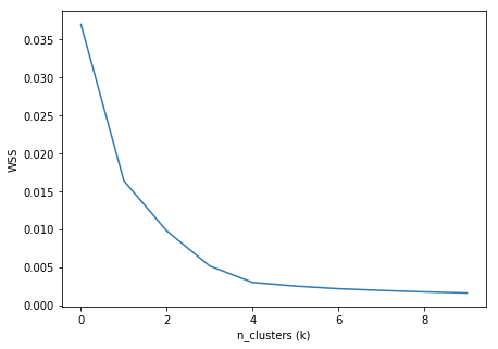
Instead of this, it was decided that we use KMeans on all the bookings at once, and use the Elbow Method to determine the optimal value of k. To find the optimal value of k, the WSS is calculated for a varying number of clusters. The total WSS measures the compactness of the clustering and we want it to be as small as possible.

Similarly, we also performed a Silhouette Analysis on the number of clusters to choose the value of k that would maximise the average silhouette score.

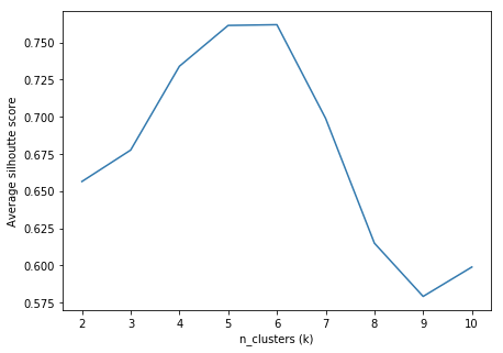
From the plots above, we can safely assume that a value of k=5 or k=6 would be the optimal value. At this point, the algorithm would choose k=6 as it has a lower WSS value for a similar Silhouette Score when compared to k=5. But looking at the silhouette plot for n_clusters=6 below it is evident that the red cluster (numbered 5) does not have a significant number of data points.

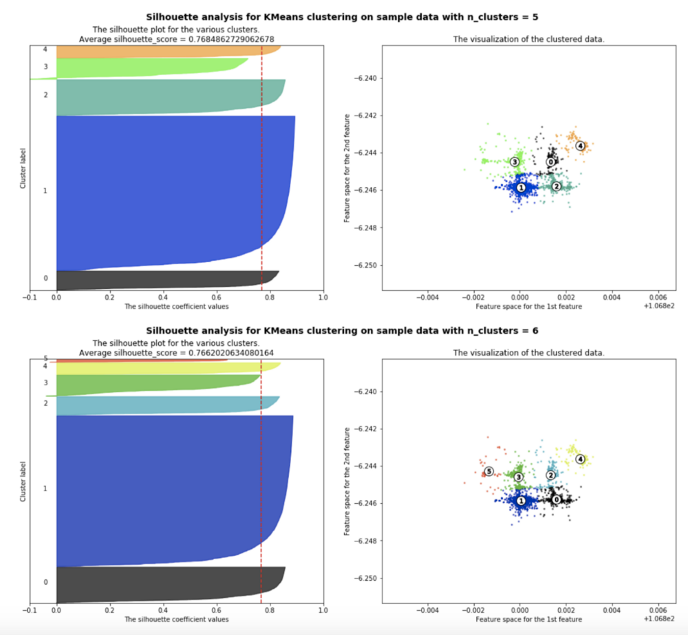
Thus, after the best value of k was determined, we used the Stupid Backoff method to make sure that the number of clusters determined really was optimum, on the basis of the significance of each cluster with respect to all pickups corresponding to that POI. Using this approach, the optimum number of clusters that was finally determined for Blok M Square was 5.

Conclusion

Once we found the number of clusters that best represented the dataset for that POI, we then assign the cluster centres (as determined by KMeans) as pickup points, or gates. But we weren’t done yet. The next step was to find the names of these gates — we had to automate this and with that came another set of challenges. How we went about naming the gates is explained in detail here.

If you found this interesting and would like to solve exciting challenges in Data Science, join us! Check out gojek.jobs for more and grab this chance to work with Southeast Asia’s first and fastest growing unicorn.